Full-Spectrum Analysis: The Optimal Method for Monetizing Information
2025-08-10
Background
How to maximize the growth rate of assets?
In 1956, J.L. Kelly published "A New Interpretation of Information Rate." The paper discussed how a gambler could use known information to maximize the compound growth rate of their assets. It proposed a probabilistic method to guide betting strategies. However, applying this paper to actual investment activities presents several issues:
- It does not utilize borrowing leverage or short selling, confining its conclusions to a practical leverage range of 0~1.
- It assumes the gambler bets on a specific event symbol, receiving a payout if it occurs next, otherwise losing the entire bet. But traders can only bet long/short, and the corresponding rise/fall events yield different results and different rates of return across different time windows.
- Liquidation timing: Kelly assumes the end of the gamble is not determined by the gambler's will. However, traders can decide to exit or continue holding at any time.
- Redundant Bayesian methods assume event development is related to prior and conditional probabilities. Removing the Bayesian framework does not affect the derived mathematical essence. It increases complexity, making direct application of the paper's formulas difficult; practical use requires simplification.
We will adopt the probabilistic method from Kelly's paper to explore a practical strategy applicable to the field of investment trading.
Full-Spectrum Analysis: FSA
Outcome Space, Optimal Leverage, and Optimal Yield
Assume implementing a certain trading strategy will ultimately result in several different outcome events. Let the outcome space be . is non-empty (in practical scenarios, there are at least 2 outcomes).
Additional assumptions:
- Deterministic Return: Each outcome event corresponds to a definite rate of return. Let the return for outcome be .
- ✅ Outcome events with different returns should be considered distinct, e.g., a 1% profit and a 2% profit are different.
- ❌ Grouping profit events with significantly different returns into the same outcome violates deterministic return.
- Deterministic Probability: Let the probability of outcome occurring be , ().
- ✅ The probability of each outcome must be deterministically assessed.
- ❌ Stating that an outcome has a likelihood of "over 80%": 80%~100% violates deterministic probability.
- Mutual Exclusivity: It is impossible for two outcomes to occur simultaneously.
- ✅ Design outcome events that are completely impossible to occur together.
- ❌ If outcome events have intersections, e.g., "holding for 20 minutes" and "falling 20%" could occur simultaneously, violating mutual exclusivity.
- Completeness: The sum of probabilities for all outcomes is 100%; there are no outcomes outside the predefined set, i.e., .
- ✅ Consider all possible outcomes that could occur.
- ❌ If the outcome events only define "rise over 20%" and "fall over 20%", but not "fluctuation between -20% and 20%", this violates completeness.
- Leverage Effect: Returns follow the leverage effect, meaning if times leverage is used, when outcome occurs, the return is , i.e., the asset becomes times its original value.
- ✅ Investment products with sufficient liquidity conform to this characteristic.
- ❌ When the position size becomes too large, market impact costs due to liquidity issues cause returns to no longer follow a linear relationship.
For the outcome space , we can calculate its Expected Earning Yield:
The concept of expected yield is intuitive and convenient to calculate. The problem with expected yield is:
- It leads to extreme decisions—either zero position or full position—failing to control bankruptcy risk. If the expected yield is positive, it tends to infinitely amplify leverage to seek higher returns, even if high leverage can lead to ruin.
- It does not consider the compounding effect. It only considers the return of a single investment, not that the market allows for repeated investments. This does not align with actual investment management scenarios.
Compound Earning Yield refers to the average yield per trade after repeating multiple independent trades:
Optimal Earning Yield is the maximum value of the compound yield across different leverage levels:
To avoid ruin (zeroing out), it must be satisfied that for all outcomes, . This leads to a basic feasible region for k:
Upper bound:
Lower bound:
And a always feasible solution ,
The optimal leverage is the within the feasible region that maximizes the compound yield .
At any moment, the actual leverage in the account can be calculated: , and the optimal leverage can be evaluated. All trading strategies ultimately correspond to an actual leverage. Making a deterministic trading decision is equivalent to determining the value of . The optimal leverage corresponds to the ideal position.
Thus, we obtain a trading framework:
- Design the outcome space .
- Continuously evaluate the probabilities of different outcomes.
- Calculate the actual leverage and the optimal leverage .
- Control the actual leverage to approach the optimal leverage.
Special Points
The trivial point , i.e., "no participation, no profit or loss." When we have no position, it is equivalent to deciding . For any instrument, whether holding a position or not, we are making a decision at every moment. Short selling corresponds to the case ; if , it means additional leverage is required.
Solving the Optimization
Recalling the problem: given outcome space , probability distribution , returns , feasible region , find the leverage ratio that maximizes the yield:
Rearranging the compound yield and taking the logarithm on both sides (preserving monotonicity), we get:
Let
According to the definition of optimal leverage:
Since is monotonically increasing:
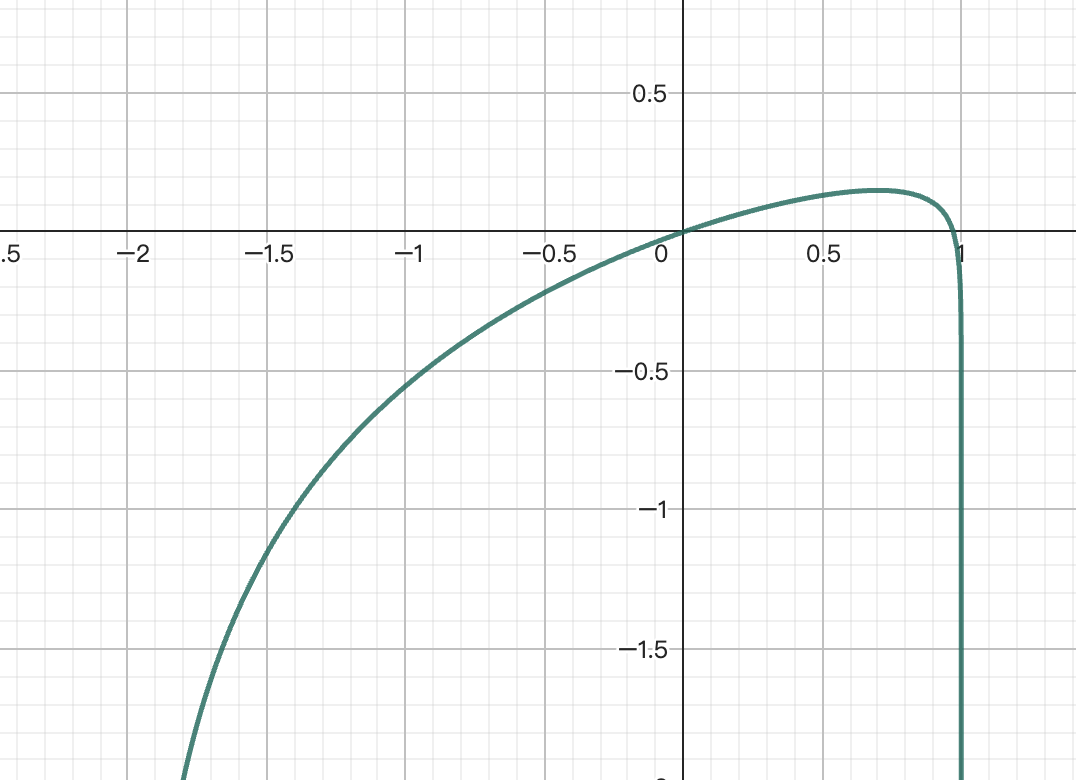
Taking the first and second derivatives of :
Each term in the second derivative is non-positive, so . If and only if , then , but in this case, , yielding no profit, which is meaningless. In other cases, . This means is a strictly concave function, and is strictly monotonically decreasing. has one and only one maximum point, and this maximum point is the global maximum.
As shown in the figure below, regardless of the number of terms, the curve of is concave.
The maximum point of is the zero of its first derivative:
If we rearrange this equation, it can be transformed into a polynomial equation in k. If there are distinct values of , the highest degree of the polynomial equation is . According to the Abel–Ruffini theorem, polynomials of degree five and higher have no general algebraic solution formula.
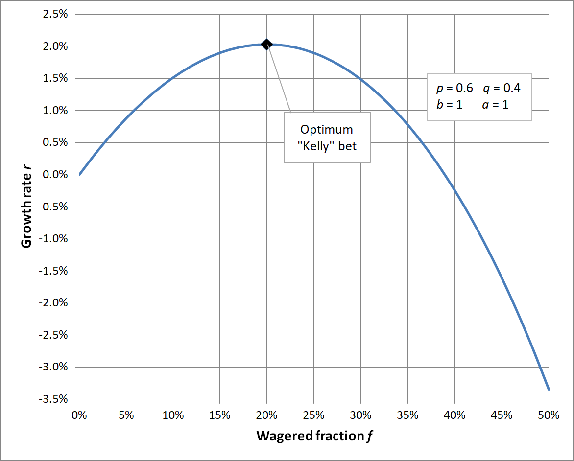
The common Kelly formula is the special case where : Let win probability be , and odds be .
| Outcome | Probability | Return |
|---|---|---|
| Win | ||
| Loss |
Substituting yields the equation:
Simplifying gives
Thus proving the Kelly formula.
For trading scenarios, there may be countless outcomes with different returns; therefore, we can only seek numerical solutions.
As a strictly concave function of a single variable, using Newton's method is the gold standard. Starting the iteration from the fixed point is a good choice; a strictly concave function will converge to the same result from any starting point.
Newton's Method Exceeding the Feasible Region
A potential issue is that the iteration point obtained by Newton's method might fall outside the problem's feasible region. A minimal example illustrates this situation:
Yielding
Calculation shows the feasible region , with analytical optimal leverage . However, when using Newton's method, the first iteration point is
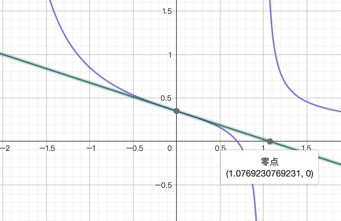
The first iteration point exceeds the feasible region, moving outside the domain where the derivative is defined, making further iteration meaningless. This shows the naive Newton's method itself cannot handle situations where it steps outside the feasible region.
The solution is to check, after calculating the next iteration point using Newton's method, whether it lies within the feasible region. If it does, iterate to that point. If not, based on its direction, take a point between the feasible region boundary and the current point as the next iteration point.
Algorithm Pseudocode
Algorithm
- Initialize
- Calculate the basic feasible region based on returns
- Clip the feasible region:
- Loop for a maximum of iterations:
- Calculate the next point:
- If is not in :
- If , set
- If , set
- If the difference is less than the precision threshold , break the loop.
- Update
- Return
Code Implementation
From a programming perspective, a more suitable abstraction is to let each outcome in the set have two attributes: return rate r and weight w. This outcome space can be traversed, and the algorithm can be written as:
/**
 * Calculates the optimal leverage k and expected return e according to the Kelly criterion.
 *
 * @param R - Array of return rates
 * @param W - Array of weights
 * @param lower - Minimum leverage constraint
 * @param upper - Maximum leverage constraint
 * @param eps - Convergence tolerance
 * @param max_iter - Maximum number of iterations
 * @param alpha - Convergence acceleration factor
 * @returns An object containing the optimal leverage k and expected return e
 */
export function resolve_k(
  R: number[],
  W: number[],
  lower = -Infinity,
  upper = Infinity,
  eps = 1e-9,
  max_iter = 100,
  alpha = 0.9
) {
  const n = R.length;
  if (n !== W.length)
    throw new Error(
      "Returning and Probability vectors must have the same length"
    );

  // Calculate the basic feasible region K, ensuring 1 + k * r > 0
  let minK = NaN;
  let maxK = NaN;
  for (let i = 0; i < n; i++) {
    const r = R[i];
    if (r === 0) continue;
    const k = -1 / r; // Critical value
    if (r > 0) minK = isNaN(minK) ? k : Math.max(minK, k);
    if (r < 0) maxK = isNaN(maxK) ? k : Math.min(maxK, k);
  }
  if (isNaN(minK)) minK = 0; // If no positive R, set minK to 0
  if (isNaN(maxK)) maxK = 0; // If no negative R, set maxK to 0
  lower = Math.max(lower, minK);
  upper = Math.min(upper, maxK);

  let sum_w = 0;
  for (let i = 0; i < n; i++) {
    const w = W[i];
    if (w < 0) throw new Error(`Weight[${i}] = ${w} must be non-negative`);
    sum_w += w;
  }
  if (sum_w === 0) throw new Error("Sum of weights must be greater than zero");

  let k = 0;
  let it;
  for (it = 0; it < max_iter; it++) {
    let acc_g1 = 0;
    let acc_g2 = 0;
    for (let i = 0; i < n; i++) {
      const r = R[i];
      const w = W[i];
      acc_g1 += (w * r) / (1 + k * r);
      acc_g2 += (w * r * r) / (1 + k * r) ** 2;
    }
    const delta_k = acc_g1 / acc_g2;
    if (!(Math.abs(delta_k) > eps)) break;
    let next_k = k + delta_k;
    if (next_k <= lower) {
      next_k = lower * alpha + k * (1 - alpha);
    } else if (next_k >= upper) {
      next_k = upper * alpha + k * (1 - alpha);
    }

    k = next_k;
  }

  const lne =
    R.reduce((acc, r, i) => acc + W[i] * Math.log(1 + k * r), 0) / sum_w;
  const e = Math.exp(lne) - 1;

  return { k, e, it, sum_w, lne, upper, lower };
}
Other Mathematical Properties
When the Feasible Region is Unbounded, a Positive Expected Yield Implies a Positive Optimal Yield
Proof: Since has the same sign as , the signs of and are the same. Consider the derivative of at : , which is precisely the expected yield . For an infinitesimal , by the definition of the derivative,
If , then there exists such that , i.e., . And the optimal yield
Q.E.D.
Furthermore, the following table can be proven:
| Expected Yield | Optimal Leverage | Optimal Yield |
|---|---|---|
| Positive | Positive | Positive |
| 0 | 0 | 0 |
| Negative | Negative | Positive |
Historical Backtesting Method for FSA
Gross Profit Margin: GPM
According to the trading framework described, at each moment, the actual leverage and the optimal leverage can be calculated, and the actual leverage should be controlled to converge to the optimal leverage.
Here, we default to using simple interest for backtesting because the compound interest model affects subsequent cost estimation. The compound interest model can cause very large changes in turnover, leading to additional market impact costs when the strategy capacity is reached. This results in the actual executable volume or cost deviating significantly from the model values, distorting the backtest. In real-world scenarios, compounding is often controlled manually, i.e., subjectively adjusting the initial equity or trading multiples to create a "partial compounding" scheme between "simple interest" and "compound interest."
Key constraint: depends only on known information at times ; no future data is used. influences the position size at time .
To perform historical backtesting, we first need the price and the corresponding planned net position size .
From a micro perspective, at time , knowing the price also means knowing the equity and the net position size .
Consider the boundary condition first: .
After a negligible analysis time, the planned net position size is obtained.
The trading volume required for adjustment is
Thereafter, until time , orders are placed immediately.
Under the assumption of sufficient liquidity, execution occurs completely at price , resulting in . Let be the cost based on turnover; then the cost is . Furthermore, the net position is affected by price changes, generating profit/loss .
In summary, at time :
In simple interest mode, both position size and transaction costs are proportional to the initial equity.
The total profit and loss (PnL) from price changes after holding is:
Total turnover:
We can estimate the maximum transaction cost the model can break even with, i.e., the Gross Profit Margin (GPM):
Subsequently, in live trading, an actual cost rate lower than this GPM is profitable. This GPM also hints at the model's capacity. A higher GPM means larger transaction slippage can be tolerated in live trading, allowing for higher actual trading volume.
The model's task is to maximize GPM, while the trading module's task is to achieve profitability under this GPM constraint. Specifically, in subsequent live trading, the trading module's task is to complete as much turnover as possible without exceeding the GPM. The trading module cannot avoid the exchange's inherent fee rate, which may be influenced by various factors such as VIP status, rebates, Maker/Taker distinctions, etc., affecting the actual fee rate. If the model's GPM is greater than an exchange's fee rate, it can be considered that the model is unlikely to be profitable on that exchange and needs improvement. If the trading module deems the current task unachievable, it can choose to reduce turnover or not trade, maintaining a zero position.
The final profit can be considered as: Turnover * (GPM - Actual Cost Rate). Increasing the initial equity will increase turnover, causing the actual cost rate to approach the GPM until it becomes unprofitable. However, from the formula, there should be an optimization problem for maximum profit. The initial equity corresponding to this maximum profit is the trading model's capacity. Specific evaluation requires further research into the relationship between turnover and cost.
Holding Resolution
In actual trading, products have a minimum trade volume step (volume_step), and positions can only be traded in integer multiples of this step. Therefore, given a floating-point target position, it cannot be tracked with 100% accuracy. We need to round this target position to a tradable position.
Holding Resolution is a positive integer.
If we apply the simple interest method to the optimal leverage and then map it via resolution, we get the target position . Substituting this into the backtesting framework yields the MER.
- If Holding Resolution = 1, it means the strategy only trades the base position. That is, the target position values are -1, 0, 1.
- If Holding Resolution = 2, it means the strategy begins to require position splitting. Target position values are -2, -1, 0, 1, 2.
- If Holding Resolution = ∞, it means the strategy can adjust the position with any precision. But this does not conform to reality.
Lower holding resolution requires less base capital for subsequent small-scale live trading, but the information utilized becomes coarser.
Theoretically, holding resolution affects turnover; lower resolution leads to lower turnover (situations that originally required adjustment become no adjustment needed). The impact of holding resolution on returns is not yet clear. Empirically, if the MER is sufficiently high and insensitive to resolution, it suggests readiness for live trading.
Live Trading Module
The live trading module needs to achieve profitability under the MER constraint.
However, the constraints for opening and closing positions are not the same. When opening, it can tolerate incomplete execution of the target turnover, but when closing, it cannot tolerate this. Therefore, closing constraints are stricter; in the worst case, market orders must be used, incurring higher fees and slippage.
Assuming the market order cost rate is , then when opening a position, it is safe to do so at a cost rate of .
For example, if MER = 0.02% and market order cost is 0.03%, then the opening cost must be at most 0.01%.
Regarding Outcome Space
Coping with Black Swan Events
A black swan event is an event that is considered extremely improbable but actually occurs.
- The probability of a black swan event cannot be estimated by any model; any estimation is futile as its probability is unknowable.
- Once a black swan event occurs, it results in enormous losses. Therefore, designing any outcome space must defend against black swan events.
- When a black swan occurs, it inevitably results in a -100% return, i.e., total loss.
- Black swan events cannot be fitted by any probability distribution using known samples. Therefore, it is necessary to assign a pseudo-probability to black swan events.
Assume we have assigned probabilities to our defined outcome space from existing samples.
We need to manually add two symmetric black swan events: . Here, 0.0013 is the probability outside in a normal distribution, approximately 1 in 770 samples. Assigning a higher probability to black swan events makes the strategy more conservative.
Designing symmetric black swan events is to avoid affecting the expected yield, preventing a change in the sign of the optimal leverage, and avoiding situations where a zero leverage scenario incorrectly suggests a short position.
The original probabilities need to be scaled down by a factor of to ensure the completeness of the new outcome space.
Adding black swan events shrinks the feasible region, strictly limiting the optimal leverage ratio to . Short selling is still possible, but additional leverage cannot be applied. Incorporating black swan events effectively prevents leverage abuse.
export function withBlackSwan(R: number[], W: number[], Pb = 0.0013) {
  const sum_w = W.reduce((acc, cur) => acc + cur, 0);
  const w_b = (Pb * sum_w) / (1 - 2 * Pb);
  return {
    R: R.concat([1, -1]),
    W: W.concat([w_b, w_b]),
  };
}
Summary
For a given outcome space , the are determined. As long as the probability distribution within the outcome space is estimated, a deterministic optimal leverage can be obtained. If you believe the trading system should be consistent, their probabilities should be repeatable. In this context, Full-Spectrum Analysis utilizes imperfect information without loss; therefore, there is no reason not to strictly follow this optimal leverage.
Some trading systems aim to find the outcome with the highest probability of occurrence and formulate trading plans based on that outcome. This is a maximum likelihood method. The risk of this approach is that if the likelihood function is relatively flat, choosing any single interpretation is insufficiently accurate. Such a strategy may appear effective at times and ineffective at others. Full-Spectrum Analysis does not need to follow the highest probability outcome; it can calculate returns under different outcomes and select the optimal position. It can capture subtle information and make optimal decisions. Thus, Full-Spectrum Analysis significantly lowers the quality threshold for monetizing information.
As for how to design the outcome space and estimate the probability distribution, that pertains to the content of the information itself that needs to be monetized. More on that next time.
